Abstract:
The methodologies employed for UV/Vis/NIR spectroscopic materials characterization will very much depend on the properties of the individual sample. The most common methods will use both a stand-alone instrument as well as an integrating sphere accessory. These basic procedures will investigate both transmission and reflectance spectra acquired in the diffuse and specular data collection formats. The spectrophotometer employed in this study is a Shimadzu UV2600 fitted with a 60 mm integrating sphere. The sphere has both a PMT and InGaAs detector for a wavelength range of 200 nm to 1400 nm.
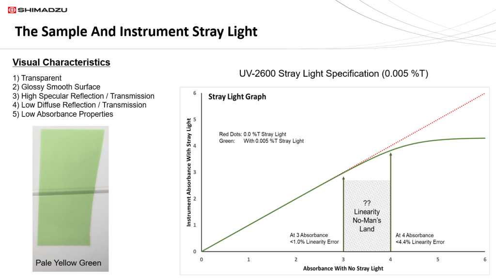
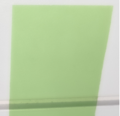
On the left is a picture of the sample used in this study, a pale yellow green gel used in stage lighting. It is a transparent thin plastic film that has a smooth specular (glossy) surface. As such, it should have high specular transmission and reflection properties. This also means that it will have low diffuse transmission and reflection properties. This film has a low concentration of dye which results in modest overall absorbance. Note how it is possible to “see through” this sample to the supporting medium below. Please remember that when using the “Mark 1” eyeball to evaluate sample properties, you are only seeing information between 380 nm to 780 nm at best. Any sample properties outside this narrow wavelength envelope must be considered unknown. (That’s why we have spectrophotometers.)
The graph on the right side shows the stray light specification for the UV-2600 instrument as a “Real verses “Measured” absorbance plot. The stray light specification, along with the signal-to-noise level, is important in that it sets the approximate upper absorbance limit for a spectrophotometer. The plot above shows how stray light not only sets the upper absorbance level, but it also is responsible for cumulative deviations from Beer’s Law. The red dotted line is the theoretical Beer’s Law relationship without any stray light affects; whereas, the solid green line has incorporated an instrumental stray light component of 0.005 %T. Note that the linear Beer’s Law relationship is maintained up to an absorbance of about 3. After a short region of increasing linearity error (the linearity no-man’s land), the measured absorbances plateau as they approach the stray light values for the instrument. A 1% linearity error is usually considered acceptable; whereas, a 5% error is considered marginal.
One last important item. An instrument’s stray light and noise does not set the upper absorbance limit in stone. It is possible to obtain data higher than the theoretical stray light plateau seen in the above plot. How can this happen? Every sample, by its wavelength dependent absorbance properties, can act as a stray light blocking filter at certain wavelengths. This means that a spectroscopist must develop certain interpretive skills to determine the presence of stray light related high absorbance artifacts in each sample.
Note that stray light photometric artifacts always yield lower than actual absorbance values.
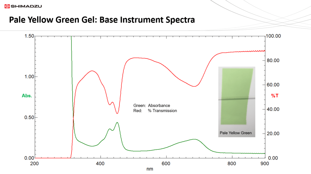
If a solid sample is thin and transparent, as this sample is, it is possible to measure it in transmission mode on a stand alone spectrophotometer. In materials characterization work one would usually start with a percent transmission spectrum. Remember that percent transmission is the “native” measurement format for any spectrophotometer; whereas, absorbance is a mathematical transformation of transmission data that linearizes it as a function of chromophore concentration. Conversion to absorbance might not be possible if there is a spectral region of extremely low percent transmission values where noise can generate negative percent transmission values. One can’t take the Log of a negative number. If there are negative values your only choice is to measure the spectrum in absorbance mode directly.
The percent transmission (red) spectrum of this sample is interesting in two respects. First it has several absorbance peaks that are responsible for its visible yellow green color. Note that in percent transmission spectra absorbance peaks are deflected downward. Second there is a sharp cut-off of light below 310 nm. This is most likely due to the absorbance of the polymer matrix of the gel. Once you have obtained a percent transmission spectrum you can always convert it mathematically to an absorbance spectrum (green). Note that in the absorbance spectrum the peaks are deflected upwards and the cut-off region below 310 nm goes off scale. A general characteristic of percent transmission and absorbance spectra is that they are typically mirror images of each other.
The usability of direct instrument transmission measurements depends on factors such as sample thickness, transparency, and chromophore concentration.
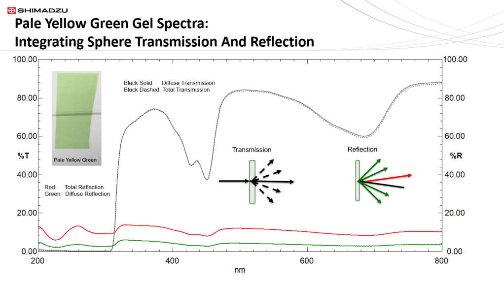
More detailed analysis can be performed if an integrating sphere accessory is available for both transmission and reflection measurements. These measurements are composed of both specular and diffuse components that together add up to a total transmission or reflection quantity.
For transmission, the specular component travels in a straight line through the sample (solid black arrows); whereas, the diffuse component is scattered by the sample through many angles (dashed black arrows). Diffuse transmission scattering occurs through 360 degrees from the incident light illumination point on the sample; however, the sphere can only collect and measure the 180 hemispherical forward scatter component.
The specular reflection component consists of light reflected at the same angle (red arrow) as the angle of incident light (black arrow). Diffuse reflection occurs throughout a 180-degree hemispherical fan (green arrows) around the incident light illumination point on the sample.
Integrating spheres can directly measure total transmission, diffuse transmission, total reflection, and diffuse reflection. In the plot shown here for the glossy, transparent film, the total (black dashed spectrum) and diffuse transmission (black solid spectrum) spectra are very close together. This is because there is minimal diffuse scatter generated from this smooth sample. Note also that the percent transmission values are relatively high due to the low dye concentration of the sample.
As we consider the reflection spectra several facts are worth discussing. The same chemical information is present in both transmission and reflection spectra; therefore they will share a similar qualitative peak structure. Reflectance spectra will, in general, be less intense than transmission spectra. This is due to the difference in path length between the two types of measurement modes. Reflectance occurs close to the sample surface with limited interior sample penetration; therefore, the pathlength is much shorter than transmission. You can see this in the region below 310 nm where the percent transmission is almost zero, but the total (red spectrum) and diffuse (green spectrum) reflection spectra retain valid information due to a shorter path length.
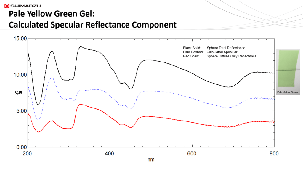
Here is a scale expansion of the reflectance spectra. As expected, the total reflection spectrum (black) is higher than the diffuse reflection spectrum (red). The difference is that the total includes the specular component. Also note the excellent spectral detail in the UV region, that was absent in the transmission spectra. Reflection spectroscopy allows for the collection of spectral data in regions where sample thickness and high absorbance prohibits a transmission measurement.
So what about the missing specular reflection data. The best way to obtain specular reflection data is with a dedicated specular reflection accessory which is designed to collect only specular data. However, if you don’t have a specular accessory you can subtract the sphere diffuse reflectance spectrum from the sphere total reflectance spectrum. The result yields an “approximation” of the specular reflection. Why approximate? Most spheres collect the diffuse reflectance by an optical geometry that allows the specular component to “escape” the sphere through one of the sphere openings. The problem is that the sphere opening is usually larger than the specular component beam. This means that a small portion of the diffuse reflection will escape along with the specular. The blue dashed line above is the specular component spectrum that results from this subtraction technique. An accurate specular measurement with a dedicated specular accessory would most likely yield a lower value of around 5 or 6 percent reflectance.
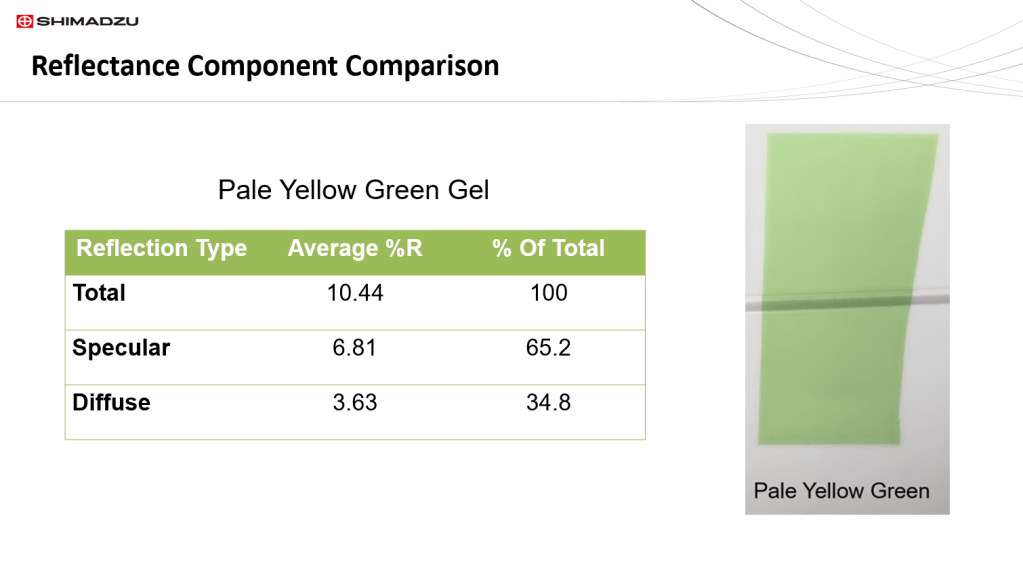
One technique for quantitatively comparing differing spectra is the spectral average method. It is nothing more than a simple average of all the spectral data points. The advantage is that it “condenses” the entire spectrum into a single number that can be compared between spectra of interest. Above is a chart of the average percent reflection by reflection type and its percentage of the total reflection. Of note is how low the diffuse reflection component is at about 3.6 percent reflection while the specular component is double the diffuse. This is due to the smooth, transparent nature of the sample.
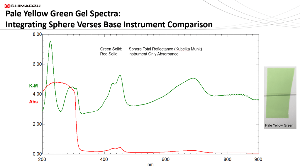
When we want to linearize transmission, we use the Beer’s Law absorbance transformation. In the world of reflectance spectroscopy we have several mathematical transformations analogous to Beer’s Law, the most common are Kubelka-Munk and Log(1/R). The Kubelka-Munk equation incorporates a scattering component. This is because it was developed to linearize reflection/concentration data from powder and paper samples where diffuse scattering is significant. In the above plot the absorbance spectrum acquired on the stand-alone spectrophotometer (red). In the region below 310 nm the absorbance is challenging the high absorbance capabilities of the instrument. Because of stray light influence, the spectrum in this region appears truncated and possibly distorted. The green spectrum is from an integrating sphere measured in total reflectance mode, then converted to Kubelka-Munk units. Note that it looks like the absorbance spectrum. We can easily see that this measurement has recovered the detail of the UV region due to the shorter path length of reflectance. Note that the entire Kubelka-Munk spectrum appears to have a large baseline offset. This is a result of the scattering component incorporated into the Kubelka-Munk equation. Since this sample doesn’t have much in the way of diffuse scattering, perhaps another type of transformation more analogous to Beer’s Law would be more realistic.
Log(1/R) is a reflectance transformation very similar to Beer’s Law absorbance derived from a transmission spectrum. In the world of reflectance one does not usually refer to absorbance, which is calculated from transmission. Rather Log(1/R) is the proper term to describe the absorbance analogue derived from reflectance measurements. It’s a small but significant point that separates the spectroscopists from the rest of the world. 🙂
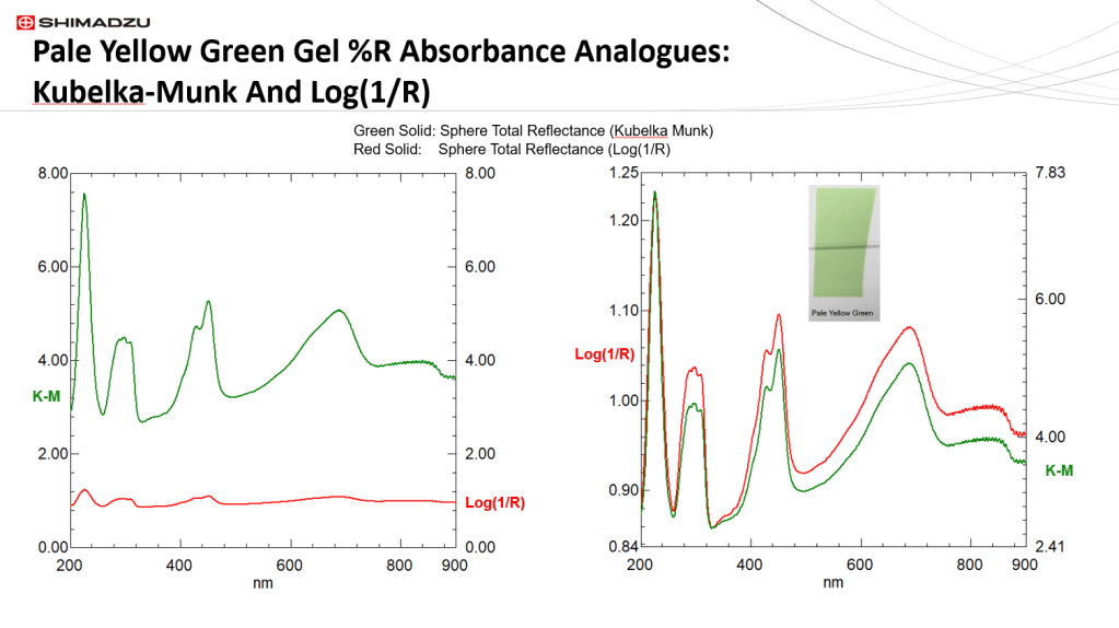
Displayed on the left side plot are the Kubelka-Munk (green) and Log(1/R) (red) spectra for the yellow green film sample. The baseline offset in the Log(1/R) is much less than the Kubelka-Munk spectrum yielding much smaller unit values that are more in line with Beer’s Law absorbance spectra. Note that both spectra have data for the UV region. The plot on the right has the two reflectance spectra normalized to closely compare peak detail. Qualitatively the two different reflectance conversions yield the same peaks with similar relative peak heights. The only striking difference between Kubelka-Munk and Log(1/R) is the baseline offset amount.
